Getting started with arrays and plots in Python

Prerequisite:

• About Python

• Setting up your Python Environment

We will learn:

• Manipulate catalog data using astropy.table.Table

• Understand data types and structures

• Learn print and f-string formatting

• Working with numpy arrays

• Plotting basic figures using matplotlib

---

# Let's start with importing our packages
import os
import numpy as np
import scipy
import matplotlib
import matplotlib.pyplot as plt
from astropy.table import Table

# We can beautify our plots by changing the matpltlib setting a little
plt.rcParams['font.size'] = 18
plt.rcParams['axes.linewidth'] = 2

Show code cell content Hide code cell content

# Let's load in the data
import os
from google.colab import drive
from astropy.table import Table

drive.mount('/content/drive/')
os.chdir('/content/drive/Shareddrives/AST207/data')

Mounted at /content/drive/

Import packages

Note how we import the packages. There are mainly 3 ways to import packages:

• directly import something, such as import matplotlib. In this way, you can call the functions under this package like matplotlib.colorbar directly.

• import something as something, such as import numpy as np. Now np is an alias of the package numpy. It is a super convenient feature and will save your life. However, there are conventions of some popular packages. E.g., import numpy as np, import pandas as pd, etc.

• import a subpackage from a package, such as import matplotlib.pyplot as plt. By doing this, we import a subpackage pyplot from matplotlib, and set up an alias plt. Another example is from astropy.table import Table, where Table is a Python class in astropy.table. Some other examples are import astropy.units as u, import astropy.constants as const.

In this notebook, we are going to learn (for the first time!) how to work with data in Python. As astronomers, a huge amount of what we do involves taking observations in the form of catalogs and comparing them visually. Today, we’re going to take a step back from space and think about football, and play around with some data for the 2023 NFL rosters.

1. Read a catalog of the football players

We have a catalog of the 2023 NFL rosters. The catalog is in the form of a CSV file, which is a common format for storing data. You can also open this CSV file using Microsoft Excel or MacOS Numbers. In Python, we can read this file using the astropy.table.Table class. We have imported this class as Table from the astropy.table package. Now we use Table.read() to read the CSV file.

cat = Table.read('./players_age.csv')
cat

Table length=1433

nflId	height	weight	birthDate	collegeName	officialPosition	displayName	height_inches	age
int64	str4	int64	str10	str30	str3	str26	float64	int64
25511	6-4	225	1977-08-03	Michigan	QB	Tom Brady	76.0	47
28963	6-5	240	1982-03-02	Miami, O.	QB	Ben Roethlisberger	77.0	42
29550	6-4	328	1982-01-22	Arkansas	T	Jason Peters	76.0	42
29851	6-2	225	1983-12-02	California	QB	Aaron Rodgers	74.0	41
30078	6-2	228	1982-11-24	Harvard	QB	Ryan Fitzpatrick	74.0	42
30842	6-6	267	1984-05-19	UCLA	TE	Marcedes Lewis	78.0	40
30869	6-7	330	1981-12-12	Louisiana State	T	Andrew Whitworth	79.0	43
33084	6-4	217	1985-05-17	Boston College	QB	Matt Ryan	76.0	39
33107	6-4	315	1985-08-30	Virginia Tech	T	Duane Brown	76.0	39
...	...	...	...	...	...	...	...	...
53053	6-3	255	1998-04-17	Memphis	DE	Bryce Huff	75.0	26
53059	6-3	239	1998-05-24	Iowa	MLB	Kristian Welch	75.0	26
53063	6-3	270	1997-10-28	Texas State	C	Aaron Brewer	75.0	27
53065	6-5	255	1997-02-22	Arizona State	TE	Tommy Hudson	77.0	27
53073	6-3	290	1997-02-28	Florida International	DT	Teair Tart	75.0	27
53074	6-3	215	1997-03-21	Indiana	WR	Nick Westbrook-Ikhine	75.0	27
53079	6-1	255	1997-08-20	Toledo	FB	Reggie Gilliam	73.0	27
53091	5-11	208	1996-05-17	Oregon State	RB	Artavis Pierce	71.0	28
53098	6-2	204	1998-03-27	Tennessee	WR	Marquez Callaway	74.0	26
53172	6-3	235	1997-06-03	Indiana State	TE	Dominique Dafney	75.0	27

This table includes many columns, including the players ID, height, weight, birthdate, etc. If you want to check all the column names, you can use cat.colnames.

cat.colnames

['nflId',
 'height',
 'weight',
 'birthDate',
 'collegeName',
 'officialPosition',
 'displayName',
 'height_inches',
 'age']

Let’s define two variables, namely height and weight:

height = cat['height_inches']
weight = cat['weight']

We note that different data have different data types. For example, the player’s name is a string, the player’s height is a float number, and the player’s weight is an integer. Data with different types might not be able to operate together. For example, you cannot add a string to a number! Some other data types include boolean, complex, etc.

Let’s check the data types of height and weight:

print("Height datatype:", height.dtype)
print("Weight datatype:", weight.dtype)

Height datatype: float64
Weight datatype: int64

Here we used the print function. The print function is used to print the specified message to the screen, or other standard output device. The message can be a string, or any other object, the object will be converted into a string before written to the screen. The arguments seperated by commas are concatenated with a space. Another very cool way of using print is to use the f-string format. You can use f before the string and use {} to include the variables. E.g., the above code can be written as print(f"Height is {cat['height'].dtype}, weight is {cat['weight'].dtype}"). This is a very convenient way to print out the variables in a string.

Let’s check the type of the height and weight columns in the catalog. They are actually astropy.table.column.Column objects.

print(f'Height column type = {type(height)}')
print(f'Weight column type = {type(weight)}')

Height column type = <class 'astropy.table.column.Column'>
Weight column type = <class 'astropy.table.column.Column'>

Often it’s more convenient to work with the data as a numpy array. We can convert the column to a numpy array using np.array(cat['height']):

height = np.array(height)
weight = np.array(weight)
print(f'height = {type(height)}')
print(f'weight = {type(weight)}')

height = <class 'numpy.ndarray'>
weight = <class 'numpy.ndarray'>

Another common way to store data is a list. A list is a collection which is ordered and changeable. In Python lists are written with square brackets. You can convert a numpy array to a list using list(). e.g.:

height_list = list(height)
print(type(height_list))
height_list[:5]

<class 'list'>

[76.0, 77.0, 76.0, 74.0, 74.0]

Exercise 1:

• Open a new cell below

• Can you find out the length of the height and weight arrays?

Tips: you can use the len() function to find out the length of an array.

for loop

A for loop is used when you have a block of code you want to repeat a fixed number of times, or iterate over a list of objects. For example, if we wanna print the first 15 elements in test_array, we can do

for i in range(15):
    print(test_array[i])

Here i stands for the index, and range(15) is a counter that starts at 0 and stops at 14.

for loop is also used when you want to iterate over a list. Let’s say we want to generate a list of players’ names. We can do the following:

names = [] # start a new empty list to store the names
for player in cat: # now we iterate over the whole catalog. `player` is a row in the catalog.
    names.append(player['displayName']) # you can append things to a list like this

Exercise 2:

Open a new cell below. Use for loop to get a list of players’ collegeName.

Indexing and slicing

Indexing refers to selecting an element from an array. Slicing refers to selecting a range of elements from an array. In Python, the index starts from 0. For example, the first element of an array is indexed as 0, the second element is indexed as 1, and so on.

If we wanna select the first element of an array, we can use array[0]. If we wanna select the forth element of an array, we can use array[3]. For the last element of an array, we can use array[-1]. The second last element of an array can be selected as array[-2].

If we wanna select the first 3 elements of an array, we can use array[0:3]. The first number is the starting index, and the second number is the ending index. The ending index is not included in the selection. If we wanna select the first 3 elements of an array, we can also use array[:3]. If we wanna select the last 3 elements of an array, we can use array[-3:]. If we wanna select every other element of an array, we can use array[::2].

Exercise 3:

Open a new cell below. Then try to select the first 5 elements of the height array, and the last 5 elements of the weight array.

2. Who’s the tallest and heaviest player?

To gain more insight into the data, let’s try to find out who’s the tallest and heaviest player in the dataset. Numpy provides a lot of useful functions to work with arrays. For example, np.max() can find the maximum value of an array; np.argmax() (argument of the max) can find the index of the maximum value in an array.

np.max(height), np.argmax(height)

(81.0, 191)

This means the tallest player is 81 inches tall, and the index of that player is 191 in the catalog. Let’s see who that player is by indexing the catalog using the index:

print(cat[np.argmax(height)])

nflId height weight birthDate  collegeName officialPosition     displayName      height_inches age
----- ------ ------ ---------- ----------- ---------------- -------------------- ------------- ---
41222    6-9    320 1988-09-22        Army                T Alejandro Villanueva          81.0  36

Exercise 4:

Find the player with the maximum weight. Is it the same as the player with the maximum height?

## Your answer goes here in this cell

3. Sort the players by height

We can sort the players by height using np.argsort(). This function returns the indices of the players from the shortest to the tallest. We can then use these indices to sort the catalog.

np.argsort(height) # Returns the indices of players sorted by height (low to high)

array([1154,  888, 1420, ...,  803,  148,  191])

height[np.argsort(height)] # indexing the original height array with the sorted indices would give us the sorted height array

array([66., 66., 66., ..., 80., 80., 81.])

This can also be achieved using the np.sort() function:

height_sorted = np.sort(height)

If you wanna get the sorted array but in the inverse order, you can use [::-1] to reverse the array.

height_sorted = np.sort(height)[::-1]
print(height_sorted)

[81. 80. 80. ... 66. 66. 66.]

Exercise 5:

Print out the weights for the players sorted by their height.

## Your answer goes here

4. Comparison and logical operations

We can use comparison operators to compare two values. The result of the comparison is a boolean value, either True or False. The comparison operators include == (equal), != (not equal), > (greater than), < (less than), >= (greater than or equal to), <= (less than or equal to). For example, 1 == 1 is True, 1 != 1 is False, 1 > 1 is False, -10 < 1 is True, 3 >= 1 is True, 1 <= 1 is True.

Sometimes we wanna combine multiple conditions. We can use logical operators to do that. The logical operators include and, or, not. For example, we can use the following:

price = 30
if price > 20 and price < 40:
    print("The price is between 20 and 40")
else:
    print("The price is not between 20 and 40")

The above code tries to check if the price is between 20 and 40. price > 20 and price < 40 is a composite condition, and it is True if the price is between 20 and 40. However, in Python, you can’t write 20 < price < 40. You have to write 20 < price and price < 40.

We also see if and else in the code. if is a conditional statement that executes some specified code after checking if the condition is True. else is a conditional statement that executes some specified code if the condition is False.

Exercise 6:

Find the number of players who have a height greater than 75 inches and a weight greater than 200 pounds.

Tip: you might wanna use np.sum(). The sum function treats True as 1 and False as 0.

## Your answer goes here

If we wanna find out how many players are taller than 75 inches and heavier than 300 pounds, we wanna combine the two conditions. We can use the & operator to combine the two conditions. The & operator is used to perform a element-wise AND operation. For example, [True, False] & [True, True] will give [True, False]. Similarly, the | operator is used to perform a element-wise OR operation. For example, [True, False] | [True, True] will give [True, True].

np.sum((height > 75) & (weight > 300))

210

Tips

See also: np.all and np.any functions.

5. Plotting the height and weight of the players

The matplotlib package is a very powerful package for plotting figures. We have imported the pyplot subpackage from matplotlib as plt. We can use plt.plot() to plot a line plot, plt.scatter() to plot a scatter plot, plt.hist() to plot a histogram, etc. Let’s first try to plot the height and weight of the players as a scatter plot.

# Your very first python plot
plt.scatter(height, weight)

<matplotlib.collections.PathCollection at 0x7da8c4eb9590>

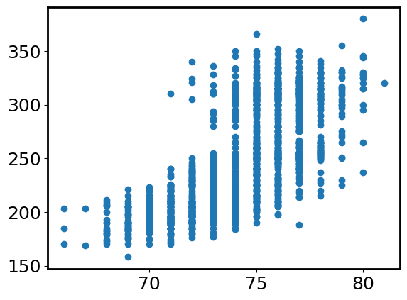
Yeah! We have our first plot. But it is not very informative. Let’s add some labels and titles to make it more informative.

plt.scatter(height, weight)
plt.xlabel('Height (inches)')
plt.ylabel('Weight (lbs)')
plt.title('Football Players')

Text(0.5, 1.0, 'Football Players')

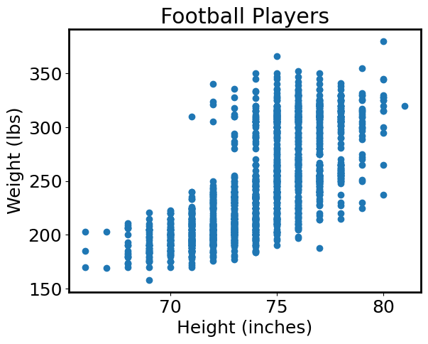
Much better! Please remember to add labels to your plots!! It is very important to make your plots informative.

You can customize the scatter plot in many ways. Please read the documentation of plt.scatter() to learn more about the customization options. We list some common options here:

• s: the size of the markers. e.g., plt.scatter(x, y, s=100) will make the markers quite large.

• c: the color of the markers. e.g., plt.scatter(x, y, c='red') will make the markers red. The color can also be an array, e.g., plt.scatter(x, y, c=age) will color the markers by the age of the players. You can also use a colormap, e.g., plt.scatter(x, y, c=age, cmap='viridis') will color the markers by the age of the players using the viridis colormap. You can find a list of colormaps here.

• marker: the shape of the markers. e.g., plt.scatter(x, y, marker='x') will make the markers crosses. Other commonly used markers include o (circle), s (square), ^ (triangle), etc. See matplotlib.markers for a full list of markers.

• alpha: the transparency of the markers. e.g., plt.scatter(x, y, alpha=0.5) will make the markers semi-transparent. The value of alpha ranges from 0 to 1, where 0 is fully transparent and 1 is fully opaque.

• label: the label of the markers. e.g., plt.scatter(x, y, label='data') will add a label to the markers. You can use plt.legend() to show the labels.

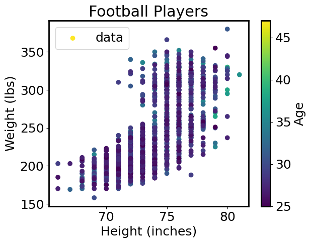
Let’s try a more sophisticated scatter plot. We will plot the height and weight of the players, and color the markers by the player’s age. We will also add a colorbar to show the age-color mapping.

height = np.array(cat['height_inches'])
weight = np.array(cat['weight'])
age = np.array(cat['age'])
plt.scatter(height, weight, c=age, label='data', cmap='viridis')
plt.xlabel('Height (inches)')
plt.ylabel('Weight (lbs)')
plt.title('Football Players')
plt.colorbar(label='Age')
plt.legend()
plt.show()

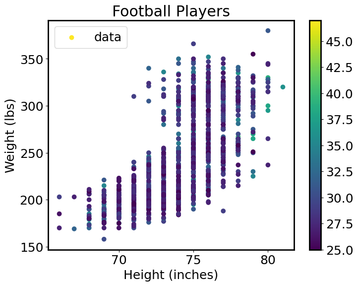
Another way to plot the above figure is to work with the matplotlib object-oriented interface. This is a more flexible way to plot figures. You can create a figure and an axis object using plt.subplots(), and then use the axis object to plot the figure. You can also add labels, titles, legends, etc. to the axis object. It will be powerful when you have multiple subplots.

We create a new figure and axis using:

fig, ax = plt.subplots()

Then we plot the figure using:

ax.scatter()

It seems a bit confusing at first, but it is actually quite simple. The plt.subplots() function creates a figure and an axis object. The fig object is the figure, and the ax object is the axis. You can use the ax object to plot the figure. For example, you can use ax.scatter() to plot a scatter plot, ax.plot() to plot a line plot, etc. You can also add labels, titles, legends, etc. to the ax object. A more complete example is shown below.

fig, ax = plt.subplots(figsize=(8, 6)) # here I set the figure size to be 8x6 inches

height = np.array(cat['height_inches'])
weight = np.array(cat['weight'])
age = np.array(cat['age'])

sct = ax.scatter(height, weight, c=age, label='data', cmap='viridis')
ax.set_xlabel('Height (inches)')
ax.set_ylabel('Weight (lbs)')
ax.set_title('Football Players')
ax.legend()

# show colorbar
cbar = plt.colorbar(sct)

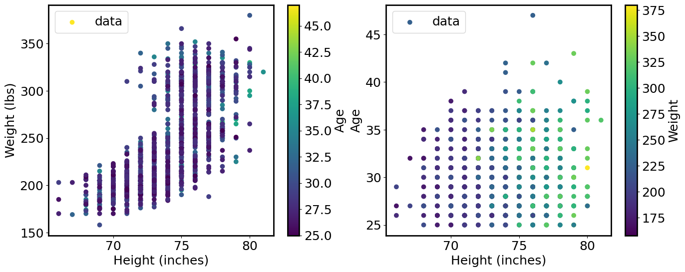
To practice your plotting skills, let’s try to plot two figures in one plot:

• left: a scatter plot of height vs. weight, color-coded by the player’s age

• right: a scatter plot of weight vs. age, color-coded by the player’s height

fig, [ax1, ax2] = plt.subplots(1, 2, figsize=(16, 6))

# left: height vs weight
sct1 = ax1.scatter(height, weight, c=age, label='data', cmap='viridis')
ax1.set_xlabel('Height (inches)')
ax1.set_ylabel('Weight (lbs)')
ax1.legend()
cbar1 = plt.colorbar(sct1, ax=ax1)
cbar1.set_label('Age')

# right: height vs age
sct2 = ax2.scatter(height, age, c=weight, label='data', cmap='viridis')
ax2.set_xlabel('Height (inches)')
ax2.set_ylabel('Age')
ax2.legend()
cbar2 = plt.colorbar(sct2, ax=ax2)
cbar2.set_label('Weight')

Tips:

You can adjust the subplots separation by using plt.subplots_adjust(). e.g., plt.subplots_adjust(wspace=0.5) will adjust the width space between the two subplots to be 0.5.

Exercise 7:

Plot a scatter plot of weight vs. age. Set the marker type to “squares”, and the marker color to orange.

Exercise 8:

Let’s calculate the BMI of these football players. BMI is defined as BMI = weight / height**2, where weight is in kg and height is in meters. The weight and height in the above data are in lbs and inches. Please convert the units, and then calculate the BMI.

Exercise 9:

Plot a scatter plot of the calculated BMI vs. age. Do you see any trend?

## Your answer here

# Your answer here

Summary

• We have learned how to read a catalog using astropy.table.Table.

• We have learned how to convert a column to a numpy array.

• We have learned how to sort an array using np.argsort().

• We have learned how to compare and combine conditions using comparison and logical operators.

• We have learned how to plot figures using matplotlib.pyplot.