Plotting JWST images

In this notebook, we will have a taste of the real data of James Webb Space Telescope. We take the images from the UNCOVER survey and plot them using python.

from matplotlib import rcParams, cycler
import matplotlib.pyplot as plt
import numpy as np
import os
import pickle
import astropy

required_packages = []  # Define the required packages for this notebook

import sys
import subprocess

try:
    import google.colab
    IN_COLAB = True
except ImportError:
    IN_COLAB = False

if IN_COLAB:
    # Download utils.py
    !wget -q -O /content/utils.py https://raw.githubusercontent.com/AstroJacobLi/ObsAstGreene/refs/heads/main/book/docs/utils.py
    # Function to check and install missing packages
    def install_packages(packages):
        for package in packages:
            try:
                __import__(package)
            except ImportError:
                print(f"Installing {package}...")
                subprocess.check_call([sys.executable, '-m', 'pip', 'install', package])
    # Install any missing packages
    install_packages(required_packages)
else:
    # If not in Colab, adjust the path for local development
    sys.path.append('/Users/jiaxuanl/Dropbox/Courses/ObsAstGreene/book/docs/')

# Get the directory right
if IN_COLAB:
  from google.colab import drive
  drive.mount('/content/drive/')
  os.chdir('/content/drive/Shareddrives/AST207/data')
else:
    os.chdir('../../_static/ObsAstroData/')

Let’s now open the JWST data!

with open('./A2744_cutoutRGB_NIRCAM.pkl', 'rb') as f:
    data = pickle.load(f)
data.keys()

dict_keys(['rIMG', 'rWCS', 'rHDR', 'rfilt', 'gIMG', 'gWCS', 'gHDR', 'gfilt', 'bIMG', 'bWCS', 'bHDR', 'bfilt'])

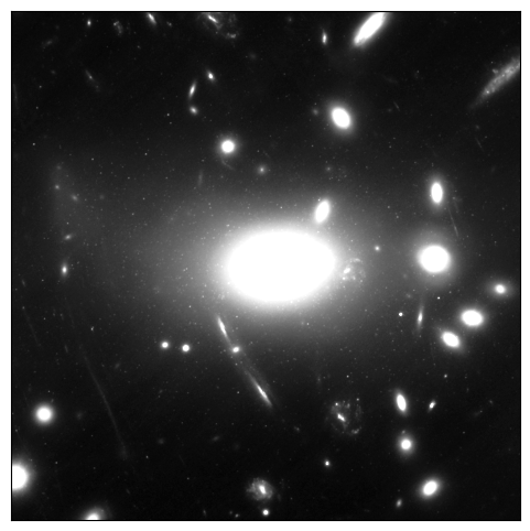
The IMG key represents the image, WCS is WCS of the image, filt is the filter name, and HDR is the image header. Let’s plot the

from utils import show_image

print('Plotting', data['bfilt'])
show_image(data['bIMG'], figsize=(6, 6), percl=0, percu=97, cmap='Greys_r')

Plotting F115W+F150W

<Axes: >

Exercise 1

Try to plot the images in other bands, and try to play with the percl and percu parameters to change the dynamical range when plotting. What are the tiny dots around the brightest cluster galaxy at the center? (just make a guess)

# your answer

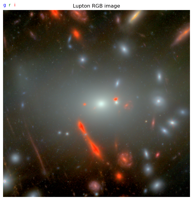
Let’s make an color-composite image for this cluster!

Black & White images are cool but a bit boring… Let’s make them colorful! Here we use the method in Lupton et al. (2004), featuring our own Robert Lupton!

from astropy.visualization import make_lupton_rgb

rgb = make_lupton_rgb(data['rIMG'], 0.85 * data['gIMG'], 1.1 * data['bIMG'], Q=10, stretch=5)

plt.figure(figsize=(8, 8))
plt.imshow(rgb, origin='lower')
plt.axis('off')

ax = plt.gca()
plt.title('Lupton RGB image')
plt.text(0.06, 1.02, 'i', transform=ax.transAxes, color='red')
plt.text(0.03, 1.02, 'r', transform=ax.transAxes, color='green')
plt.text(0, 1.02, 'g', transform=ax.transAxes, color='blue')

Text(0, 1.02, 'g')

Exercise 2

1. There are three parameters in the lupton_rgb function: stretch, Q, and minimum. Try to play with these parameters, and find a combination that makes the most beautiful color image.

2. Why are a few galaxies so red in the above image?

## your answer