
Setting up Your Python Environment#
Tip
TL;DR: There are two main ways to set up your Python environment for this course:
Work on Google Colab (recommended)
Work on your local machine
Google Colab#
Google Colab allows you to run Python notebook in the cloud with zero installation locally on your computer. What you need is only a Google account, and you can start coding right away on your browser.
Pros:
No installation required
Free to use
Can run on any device with a browser
Easy to share and collaborate with others (good for your final project)
Cons:
It may not be as fast as running on your local machine
You may need to upload/download files to/from Google Drive, and download the notebook for submission.
Recommended Workflow for Colab#
To work on the Jupyter notebooks provided in this book and submit your completed work, please follow the steps below:
1. Open the Notebook in Google Colab#
Navigate to the desired notebook in this Jupyter Book.
At the top of the notebook page, click on the rocket icon and then click the “Colab” button. This will launch the notebook in Google Colab, where you can interactively work on it.
2. Save a Copy to Your Google Drive#
In Google Colab, go to the menu and select File → Save a Copy in Drive. This will create a personal copy of the notebook in your Google Drive, ensuring you can edit and save your work. We suggest you to make a folder for all the notebooks you will work on, and save your progress regularly.
If you see a warning that “This notebook was not authored by Google,” you can click on “Run Anyway” to proceed.
3. Work on the Notebook#
Complete the tasks, exercises, or questions in the notebook as instructed.
Make sure all cells are executed, and your results are correctly displayed.
4. Download and Submit Your Work#
Once you’ve completed the notebook, download two versions of your work for submission:
ipynb(Jupyter Notebook): Go to File → Download → Download .ipynb to get the notebook file.PDF Version: Go to File → Print or File → Save as PDF to export your notebook as a PDF.
Ensure all code cells, outputs, and any written explanations are visible in the PDF.
Submit both the
.ipynbfile and the PDF file through Canvas.
Local Machine (most likely your laptop)#
If you prefer to work on your local machine, you need to properly set up your Python environment and install the necessary packages. Some of the instructions below are borrowed from Peter Melchior.
If you use Windows#
Please follow these instructions for installing the Windows Subsystem for Linux (WSL) - Ubuntu: https://docs.microsoft.com/en-us/windows/wsl/install-win10
Install Git. Open your command prompt, type “bash” to start a bash shell. Then run the following commands (you may need to type your computer login password):
sudo apt update
sudo apt install git
sudo apt install wget
Install Anaconda for Linux with Python 3.12 (note: not Anaconda for Windows!). To do this, in your command prompt, again make sure you are in the bash shell (if you still have the window open from the last step, use that, or type “bash” in a new command prompt). Then run:
wget https://repo.anaconda.com/archive/Anaconda3-2024.10-1-Linux-x86_64.shTo execute the script, type:
./Anaconda3-2024.10-1-Linux-x86_64.sh
If it doesn’t execute, you need to change the access permissions and make it executable:
chmod 755 Anaconda3-2024.10-1-Linux-x86_64.sh
To access the content of your Linux distribution from your windows interface you should follow the steps described on this website. The summary is as follows:
Go to your home directory (e.g.
C:\Users\remyj) on windows with your usual graphical interface. Among the tabs on the top right click View and tick the Hidden items box, then openAppData\Local\PackagesIn there you should find a file with a name like
CanonicalGroupLimited.Ubuntuxxxxxxxxx.Once in there, go to
LocalState\rootsf\homeand you should see your home directory.To do the converse operation and see your windows files from you Ubuntu prompt, you may do so by typing in your Unix prompt:
cd /mnt/c/Users/remyIf Anacanda stops working in your Ubuntu environment, you need to load your
.bashrcagain:source ~/.bashrc
Note
You will likely need help from us to set up your Python environment. Please let us know if you need help.
If you use Linux or MacOS#
MacOS#
Please make sure you have the command-line tools installed. Open the Terminal program and run the following command:
xcode-select --install
Install Anaconda for Mac from the Anaconda website
Linux#
Simple: Open a terminal, and stat from step 3 above for Windows.
Jupyter Notebooks#
Jupyter notebooks are one of the many possible ways to interact with Python and the scientific libraries. We like them because they are:
browser-based and interactive
easy to share with others
easy to combine code, text, and figures, especially with Markdown
compatible with Google Colab
We will be using Jupyter notebooks for all the coding exercises in this course.
Figure 2 shows the execution of some code (borrowed from here) in a Jupyter notebook locally on a web browser. Figure 3 shows the “welcome” notebook in Google Colab.

Fig. 2 Jupyter notebook viewed locally on a web browser#
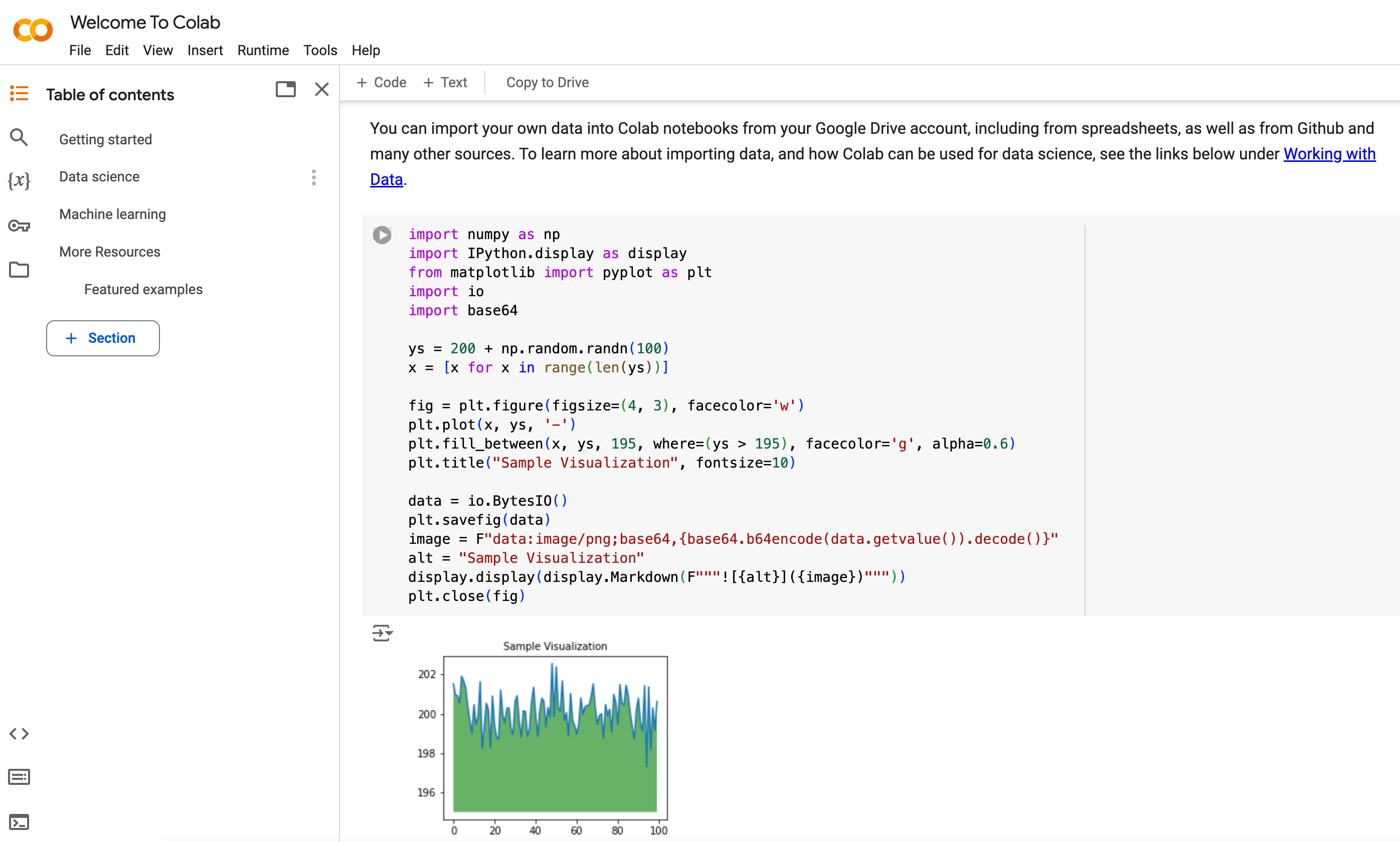
Fig. 3 Jupyter notebook viewed in Google Colab#
While Jupyter isn’t the only way to code in Python, especially when you have to run jobs on large datasets, do large numerical simulations, or run machine learning models. However, it’s great to get started with Python and learn the basics of programming and data analysis.
Starting the Jupyter Notebook#
This only applies if you are working on your local machine.
Once you have installed Anaconda, you can try to open up a terminal and type jupyter notebook in the folder you want to work at. This will open a new tab in your default web browser with the Jupyter dashboard. The output in the terminal would tell you that the notebook is running at http://localhost:8888/. localhost refers to your local machine, and 8888 is the port number on your computer.
You can then navigate to the folder where you have saved the notebooks and open them.
Assuming all this has worked OK, you can now click on New at the top
right and select Python 3 or similar. This will open a new notebook.
If you are working on Google Colab, you can simply open the notebook in the browser and start working on it.
Notebook Basics#
Let’s start with how to edit code and run simple programs. The demonstration below is done in Google Colab, but the same principles apply to Jupyter notebooks on your local machine. This video provides a good introduction to Jupyter notebooks.
Running Cells#
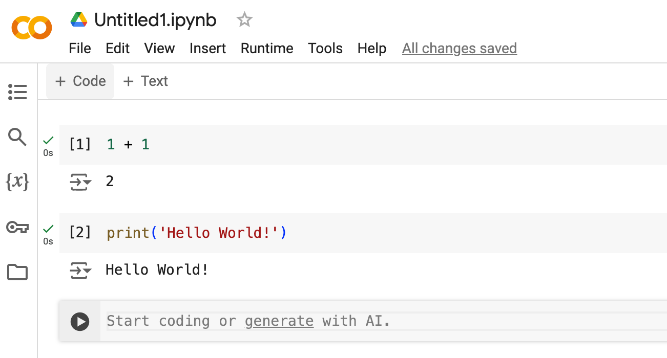
Each “cell” here is a little snippet of code. The number [1] on the left of the first cell indicates that this is the first cell run so far.
You can run each cell by clicking the little “play” button on the left side of the cell, or by pressing Shift+Enter on your keyboard.
When you click inside a cell, the cell will be in the edit mode, and you’ll see a flashing cursor. When you run the cell, the code will be executed, and the output will be displayed below the cell.
Modal Editing#
The next thing to understand about the Jupyter notebook is that it uses a modal editing system.
This means that the effect of typing at the keyboard depends on which mode you are in.
The two modes are
Edit mode
Indicated by a blinking cursor
Whatever you type appears as is in that cell
Command mode
No blinking cursor
Keystrokes are interpreted as commands — for example, typing
badds a new cell below the current one;dddeletes the current cell. Understanding these shortcuts can speed up your workflow.
To switch to
edit mode to command mode: either click outside the cell, or hit the
Esckeycommand mode to edit mode: click in a cell
Tab Completion#
In the figure above, we executed the line import numpy as np
NumPy is a numerical library we’ll work with in depth.
After this import command, functions in NumPy can be accessed with
np.function_name type syntax.
For example, try
np.random.randn(3).
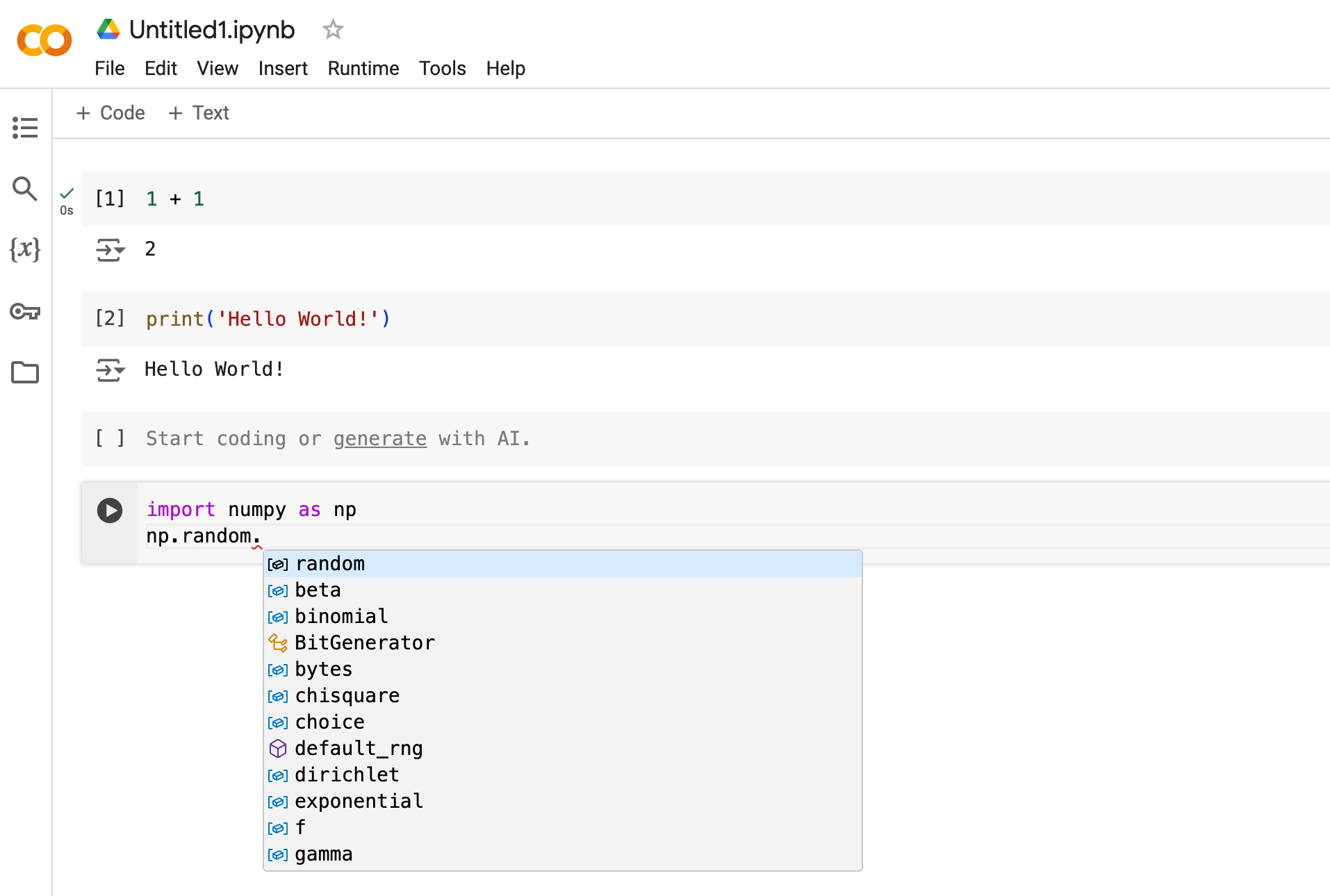
We can explore these attributes of np using the Tab key.
For example, here we type np.random. and hit Tab, Jupyter offers many completions, as shown in the figure above.
In this way, the Tab key helps remind you of what’s available and also saves you typing.
This trick is useful because you can’t possibly remember all the functions and methods available in the libraries you use. Also it helps you avoid typos. Please try this yourself!!
On-Line Help#
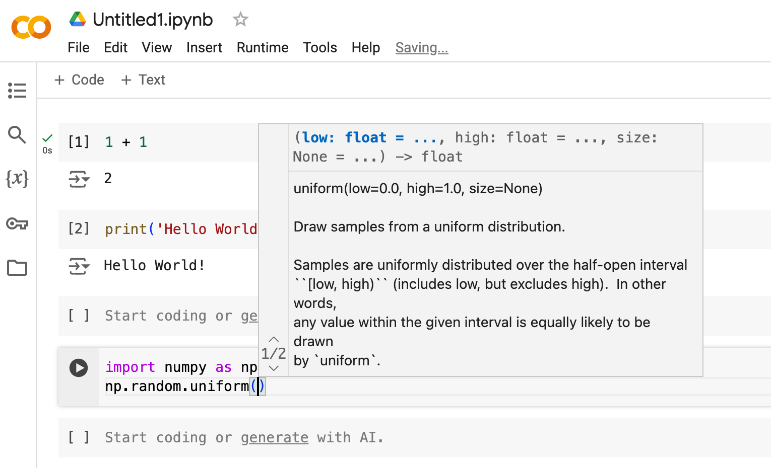
To get help on np.random.uniform, say, we can do:
Execute
np.random.uniform?: This will open a separate pane at the bottom/right of the screen with the documentation string for the function.Type
np.random.uniform()and thenShift+Tabwhen your cursor is in the middle of(|): This will show the same documentation string in a pop-up window. I personally prefer this method because it’s faster.
When you need to view the complete documentation, you can do np.random.uniform?? to open a new tab with the source code of the function.
Markdown Cells#
Another nice feature of Jupyter notebooks is that you can write text, equations, and figures in Markdown cells. Markdown is a simple language for formatting text. To insert a new Markdown cell on google colab, move your cursor between two cells and click on the + Text button that appears (or Insert -> Text cell).
Some of the most common Markdown commands are:
#for headers (smaller headers have more#s)*or-for bullet points1.for numbered lists**bold**for bold text*italic*for italic text[link](http://url)for links$$for equations, such as$$\int_0^\infty x^2 dx$$
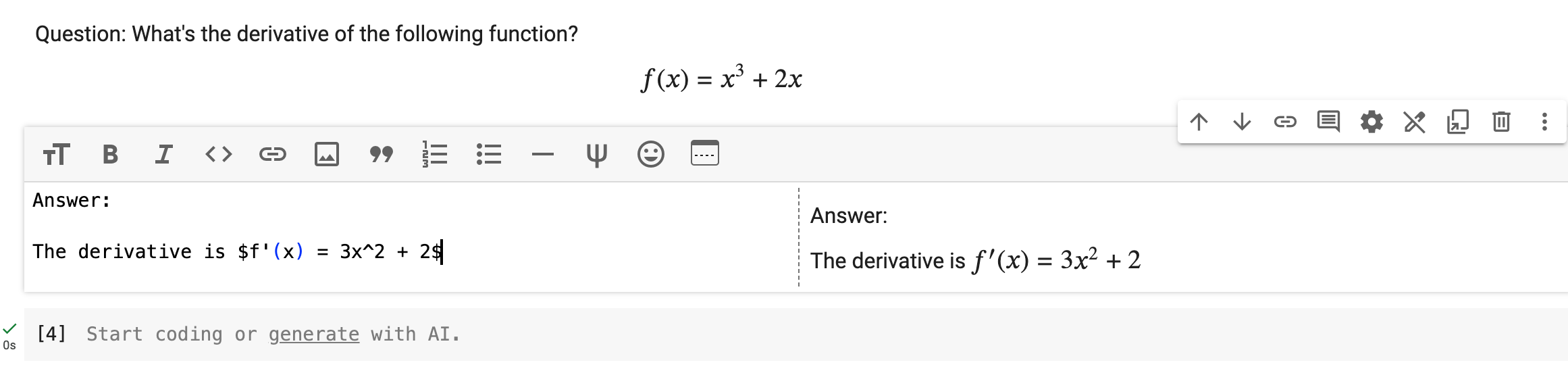
We will ask you to write down you answers to homework questions in Markdown cells. For example:
A Test Program#
Let’s run the following program to plot a histogram of 1,000 draws from a standard normal random variable. Please copy the code below to a new cell in your Jupyter notebook and run it.
import matplotlib.pyplot as plt
import numpy as np

# Fixing random state for reproducibility
np.random.seed(19680801)

n = 100_000
x = np.random.standard_normal(n)
y = 2.0 + 3.0 * x + 4.0 * np.random.standard_normal(n)
xlim = x.min(), x.max()
ylim = y.min(), y.max()

fig, (ax0, ax1) = plt.subplots(ncols=2, sharey=True, figsize=(9, 4))

hb = ax0.hexbin(x, y, gridsize=50, cmap='inferno')
ax0.set(xlim=xlim, ylim=ylim)
ax0.set_title("Hexagon binning")
cb = fig.colorbar(hb, ax=ax0, label='counts')

hb = ax1.hexbin(x, y, gridsize=50, bins='log', cmap='inferno')
ax1.set(xlim=xlim, ylim=ylim)
ax1.set_title("With a log color scale")
cb = fig.colorbar(hb, ax=ax1, label='counts')

plt.show()
Don’t worry about the details for now — let’s just run it and see what happens. Hopefully you will get a beautiful plot!
Homework#
Set up your Python environment, either on Google Colab, or on your own laptop. If you are working on your local machine, please make sure you can run a Jupyter notebook. If you are working on Google Colab, please make sure you can open a notebook and run the code.
Familiarize yourself with the Jupyter notebook interface. Try running some code, writing some text, and inserting a figure in a Markdown cell.
Run the test program above and make sure you get a plot. If you encounter any errors, please let us know.
Download the notebook as
.ipynband print it as a PDF. Submit both files through Canvas.