
Part 3 Lightcurves#
Assumed knowledege:
CCD operation and structure
Point-spread functions
Plotting tools
Model fitting
Step 0: imports#
# Run this once to install a python package for downloading lightcurves from the TESS mission
# ! python -m pip install lightkurve --upgrade
# these should be familar
import scipy
import numpy as np
import pandas as pd

import matplotlib
import matplotlib.pyplot as plt

# this package will allow us to make progress bars
from tqdm import tqdm

# We can beautify our plots by changing the matpltlib setting a little
plt.rcParams['font.size'] = 18
matplotlib.rcParams['axes.linewidth'] = 2
matplotlib.rcParams['font.family'] = "serif"
Step 1: loading data from the TESS mission#
Like the last notebook, the function below uses the python package lightkurve to load data from the TESS mission. To search for exoplanets, TESS takes pictures of a patch of the sky once every 2 minutes. The function load_TESS_data takes in the name of a star and the size of image cutout we want to downdload (centered on the star).
Exercise: Run the code below to load in the functions we used in the last notebook.
# this function downloades TESS lightcurves (I recommend we supply this function
# and have the student's use it as a black box)

def load_TESS_data(target, cutout_size=20, verbose=False, exptime=None):
    """
    Download TESS images for a given target.

    inputs:
        target: str, same of star (ex. TOI-700)
        cutout_size: int, size of the returned cutout
                     (in units of pixels)
        verbose: bool, controls whether to include printouts
        exptime: str, determines if we use short or long cadence mode
                 (if None, defaults to first observing semester)
    outputs:
        time: numpy 1D array
        flux: numpy 3D array (time x cutout_size x cutout_size)
    """

    import lightkurve as lk

    # find all available data
    search_result = lk.search_tesscut(target)
    if exptime == 'short':
        search_result = search_result[search_result.exptime.value==search_result.exptime.value.min()]
    elif exptime == 'long':
        search_result = search_result[search_result.exptime.value==search_result.exptime.value.max()]
    print(search_result)

    # select the first available observing sector
    if exptime:
        search_result = search_result[search_result.exptime == exptime]
    search_result = search_result[search_result.mission == search_result.mission[0]]

    # download it
    tpf = search_result.download_all(cutout_size=cutout_size)[0]

    # convert it to a numpy array format
    flux = np.array([
        tpf.flux[i].value for i in range(len(tpf.flux)) if tpf.flux[i].value.min()>0
    ])
    flux_err = np.array([
        tpf.flux_err[i].value for i in range(len(tpf.flux_err)) if tpf.flux[i].value.min()>0
    ])

    time = np.array([
        tpf.time.value[i] for i in range(len(tpf.flux)) if tpf.flux[i].value.min()>0
                    ])

    return time, flux, flux_err
def plot_cutout(image, logscale = False, vrange = [1,99]):
    """
    Plot 2D image.

    inputs:
        image: 2D numpy array
        logscale: bool, if True plots np.log10(image)
        vrnge: list, sets range of colorbar
               (based on percentiles of 'image')
    """
    if logscale:
        image = np.log10(image)

    q = np.percentile(image, q = vrange)
    plt.imshow( image, vmin = q[0], vmax = q[1] )
    plt.show()

def psf(x,y,sigma,scale,bkg,xmu=0,ymu=0,unravel=False):
    """
    Symmetric 2D point-spread function (PSF)

    inputs:
        x: np.ndarray, where to evaluate the PSF
        y: np.ndarray, where to evaluate the PSF
        sigma: float, width of the PDF
        scale: float, integrated area under the PSF
        bkg: float, background flux level
        xmu: float, center of PSF in x
        ymu: float, center of PSF in y
    outputs:
        PSF evalauted at x and y
    """
    exponent = (np.power(x-xmu,2) + np.power(y-ymu,2) ) / sigma**2

    mod = scale * np.exp(-exponent) / (2*np.pi*sigma**2) + bkg
    if unravel:
        return mod.ravel()
    else:
        return mod

def residual(theta, x, y, z, z_err):
    sigma, scale, bkg, xmu, ymu = theta

    model = psf(x,y,sigma=sigma,scale=scale,bkg=bkg,xmu=xmu,ymu=ymu)

    chi = np.power(model - z,2)/z_err**2

    return np.sum(chi)
Exercise: Run the code below to load all the TESS data for one small patch of the sky. We’ll center our images on the same variable star from the last notebook.
target = 'Gaia_DR2279382060625871360'
cutout_size = 20 # dimensions of the image in pixels x pixels
time, flux, flux_err = load_TESS_data(target,verbose=True,cutout_size=cutout_size)
SearchResult containing 4 data products.

 #     mission     year  author exptime        target_name         distance
                                   s                                arcsec
--- -------------- ---- ------- ------- -------------------------- --------
  0 TESS Sector 19 2019 TESScut    1426 Gaia_DR2279382060625871360      0.0
  1 TESS Sector 59 2022 TESScut     158 Gaia_DR2279382060625871360      0.0
  2 TESS Sector 73 2023 TESScut     158 Gaia_DR2279382060625871360      0.0
  3 TESS Sector 86 2024 TESScut     158 Gaia_DR2279382060625871360      0.0
# where to evaluate our PSF
x = np.arange(flux.shape[1])
y = np.arange(flux.shape[2])
X,Y = np.meshgrid(x,y)
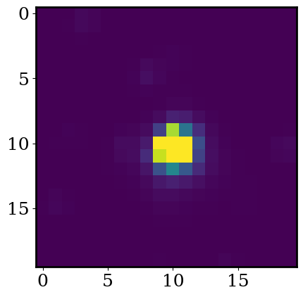
Exercise: To check things loaded well, run the code below to plot the mean of the TESS cutouts.
# linear scale
plot_cutout(np.mean(flux,axis=0))
Exercise: As a refresher, first plot the total flux in each cutout as a function of time. Remember, this is the simple light curve we made in the last notebook. Be sure to label your plot.
# answer here
Exercise: Now let’s measure the flux of the cutouts using our more robust method. With your code from the end of the last notebook, use scipy.optimize.minimize to find the best-fit scale for each TESS cutout.
Plot the light curve.
# answer here
Step 3: finding the oscillation period#
We’ve now successfully made a lightcurve for our star! By eye we can see the star is variable (it’s flux is periodically varying with time).
Exercise: By eye, how long does it take for the star’s flux to complete a cycle?
answer here
Now let’s try to measure the oscillation period. We’ll start by fitting the lightcurve with a simple periodic function: a sine wave.
Exercise: Write the function sinusoid_model(time,ampl,period,phase,background) where time is a numpy array, and ampl,period,phase,background all all floats. The function shound return:
$\( y(t) = A \sin[t \times (2\pi / \mathrm{period})+ \mathrm{phase}] + \mathrm{background} \)$
As a test, sinusoid_model(time=0.1,ampl=2,period=2,phase=0.1,background=1) should return 1.8045.
# answer here
Exercise: Plot the sine wave alongside the lightcurve we calculated above (with scipy). Set the parameters of sinusoid_model by hand to best fit the lightcurve.
# answer here
Now let’s try automating the process.
Exercise: For a grid of periods (0 < period < 5) and phases (0 < phase < 2 * np.pi), calculate the goodness of fit:
np.sum(np.power(lightcurve-model,2) ). For each combination of period and phase, plot period versus phase on a scatter plot with the color of the marker set by np.log10 of goodness of fit. Leave ampl=100 and background=600.
For ease of reading, try setting your colorbar to go from vmin = 6. and vmax=7.3
# answer here
Exercise: Compare the best fit sine wave with the lightcurve.
# answer here
Our sine model works okay but certainly isn’t a perfect fit to the data. Instead let’s try a Lomb-Scargle periodogram. This method finds the periodic signals in a dataset using Fourier transforms. See some background: https://iopscience.iop.org/article/10.3847/1538-4365/aab766/pdf
Exercise: Run the code below to calculate the Lomb-Scargle periodogram. Plot period vs. power. Use a log scale on the x-axes.
This tell us how much a particular period contributes to the observed signal (so spikes tell us that period is strongly present in the data).
from astropy.timeseries import LombScargle

periods   = 10**np.linspace(np.log10(2),2,1000)
frequency = 1/periods
power = LombScargle(time,lightcurve).power(frequency)
plt.plot(periods,power)
_ = plt.xlabel('Period [days]')
_ = plt.ylabel('Power')
plt.xscale('log')
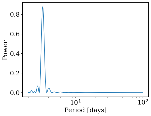
best_period = periods[np.argmax(power)]
print(f'Best: {best_period:.3} days')
Best: 3.29 days
Exercise: How does the peak from the Lomb-Scargle periodogram compare to the best fit period you found with out sine function above?
answer here
Step 4: finding planets#
Above we measured the lightcurve for a star from TESS cutouts and then calculated it’s oscillation period. Let’s now repeat that process for a star known to host a transiting planet!
Let’s consider a relatively bright star hosting a Jupiter sized planet:
Exercise: Run the code below to load the TESS data.
target = 'Gaia_DR24624979393181971328'

period_tess = 2.084544     # days
radius_star_tess   = 1.17  # R_sun
cutout_size = 20 # dimensions of the image in pixels x pixels

# stamps
time, flux, flux_err = load_TESS_data(target,verbose=True,cutout_size=cutout_size,exptime=158)
SearchResult containing 36 data products.

 #     mission     year  author exptime         target_name         distance
                                   s                                 arcsec
--- -------------- ---- ------- ------- --------------------------- --------
  0 TESS Sector 06 2018 TESScut    1426 Gaia_DR24624979393181971328      0.0
  1 TESS Sector 05 2018 TESScut    1426 Gaia_DR24624979393181971328      0.0
  2 TESS Sector 04 2018 TESScut    1426 Gaia_DR24624979393181971328      0.0
  3 TESS Sector 03 2018 TESScut    1426 Gaia_DR24624979393181971328      0.0
  4 TESS Sector 01 2018 TESScut    1426 Gaia_DR24624979393181971328      0.0
  5 TESS Sector 02 2018 TESScut    1426 Gaia_DR24624979393181971328      0.0
  6 TESS Sector 13 2019 TESScut    1426 Gaia_DR24624979393181971328      0.0
  7 TESS Sector 11 2019 TESScut    1426 Gaia_DR24624979393181971328      0.0
  8 TESS Sector 12 2019 TESScut    1426 Gaia_DR24624979393181971328      0.0
  9 TESS Sector 08 2019 TESScut    1426 Gaia_DR24624979393181971328      0.0
 10 TESS Sector 07 2019 TESScut    1426 Gaia_DR24624979393181971328      0.0
 11 TESS Sector 09 2019 TESScut    1426 Gaia_DR24624979393181971328      0.0
 12 TESS Sector 27 2020 TESScut     475 Gaia_DR24624979393181971328      0.0
 13 TESS Sector 33 2020 TESScut     475 Gaia_DR24624979393181971328      0.0
 14 TESS Sector 30 2020 TESScut     475 Gaia_DR24624979393181971328      0.0
 15 TESS Sector 32 2020 TESScut     475 Gaia_DR24624979393181971328      0.0
 16 TESS Sector 31 2020 TESScut     475 Gaia_DR24624979393181971328      0.0
 17 TESS Sector 28 2020 TESScut     475 Gaia_DR24624979393181971328      0.0
 18 TESS Sector 29 2020 TESScut     475 Gaia_DR24624979393181971328      0.0
 19 TESS Sector 39 2021 TESScut     475 Gaia_DR24624979393181971328      0.0
 20 TESS Sector 36 2021 TESScut     475 Gaia_DR24624979393181971328      0.0
 21 TESS Sector 37 2021 TESScut     475 Gaia_DR24624979393181971328      0.0
 22 TESS Sector 38 2021 TESScut     475 Gaia_DR24624979393181971328      0.0
 23 TESS Sector 34 2021 TESScut     475 Gaia_DR24624979393181971328      0.0
 24 TESS Sector 35 2021 TESScut     475 Gaia_DR24624979393181971328      0.0
 25 TESS Sector 68 2023 TESScut     158 Gaia_DR24624979393181971328      0.0
 26 TESS Sector 69 2023 TESScut     158 Gaia_DR24624979393181971328      0.0
 27 TESS Sector 67 2023 TESScut     158 Gaia_DR24624979393181971328      0.0
 28 TESS Sector 66 2023 TESScut     158 Gaia_DR24624979393181971328      0.0
 29 TESS Sector 61 2023 TESScut     158 Gaia_DR24624979393181971328      0.0
 30 TESS Sector 65 2023 TESScut     158 Gaia_DR24624979393181971328      0.0
 31 TESS Sector 64 2023 TESScut     158 Gaia_DR24624979393181971328      0.0
 32 TESS Sector 63 2023 TESScut     158 Gaia_DR24624979393181971328      0.0
 33 TESS Sector 62 2023 TESScut     158 Gaia_DR24624979393181971328      0.0
 34 TESS Sector 87 2024 TESScut     158 Gaia_DR24624979393181971328      0.0
 35 TESS Sector 88 2025 TESScut     158 Gaia_DR24624979393181971328      0.0
Exercise: To get acquainted with this star, first use plot_cutout to plot the first image (i.e., flux[0]).
# answer here
Exercise: Now let’s measure a simple light curve. Plot the total flux in each cutout as a function of time. Be sure to label your plot.
# answer here
Exercise: Next use scipy.optimize.minimize to extract the lightcurve from the TESS cutouts by fitting the images with the 2-d gaussian model. Just like we did at the end of the last notebook.
Use the ranges for the parameters from the last notebook: (.1,5) for sigma, (0,1000) for scale, (0,10) for bkg, (5,15) for xmu and ymu.
Hint: set the initial guess for x0 = [1, 40, 0.1, cutout_size/2, cutout_size/2].
Plot the lightcurve.
# answer here
Exercise: What do you notice about the lightcurve? Can you spot transits by eye? How does the lightcurve using scipy compare to the simple “total flux” lightcurve?
answer here
In addition to transits, we can also see the star is undergoing a more steady change in brightness with time. We want to study the transits so let’s try to remove the non-transit flux changes (this is called “detrending” the lightcurve).
Let’s use the function median_filter(x,y,width), where x,y are arrays (for example time and lightcurve) and width is a float, to detrend the lightcurve. For each x value, the function returns with the median y within width of the given x value (i.e., a rolling median filter).
Exercise: Run the code below to load the median_filter function. Then evaluate median_filter on the lightcurve we measured with scipy, set width=1.
def median_filter(x,y,width):
    smooth = []
    for xi in x:
        C = np.abs(xi-x)<width/2
        smooth.append(np.median(y[C]))
    return np.array(smooth)
# answer
Exercise: On the same plot, compare the lightcurve the median filter. Show the median filter for different values of width. Try width between 0.1 and 10.
# answer
Exercise: For which value of width does the median filter best match the long-period changes in the lightcurve and not trace the transits? Remember we want to use the median filter to remove the long term trends without affecting the transits.
answer here
Exercise: Detrend the lightcurve by subtracting median_filter (with your chosen width). Call the detrended lightcurve lc_detrended
Plot the detrended lightcurve.
# answer here
Exercise: Now use calculate the Lomb-Scargle periodogram for our cleaned light curve. Plot period vs. power. Be sure to label your plot.
Let’s look at periods = 10**np.linspace(np.log10(1.1),2,1000); this means we are looking for periodic signals between \(1.1\) and \(100\) days. Also remember, the LombScargle function takes in frequency = 1/periods.
# answer here
Exercise: At what period is the power of the Lomb-Scargle periodogram greatest? Call this period.
hint: use np.argmax
# answer here
We now have a clean lightcurve and a solid estimate of the planet’s orbital period. So we have everything we need to study the planet! Unfortunately, this is difficult with individual transits, because each transit is quite a noisy measurement. We can overcome this challenge by combining the individual transits into one ‘average’ transit.
Exercise: Since the planet’s orbital period is constant, the transit times should follow a simple formula:
$\( T(n) = T_0 + P \times n \)\(
where \)T(n)\( is the \)n\(th transit time (i.e., \)n=0,1,2,\dots\(), \)T_0\( is the first observed transit time, and \)P$ is the orbital period.
This means we can “fold” all the individual transits on top of each other to create a higher signal average transit, if we know the planet’s period.
Use the provided function phase_it to fold the light curve to the Lomb-Scargle period and plot the folded lightcurve. Change the x limits to zoom in on the transit. Be sure to use the detrended light curve.
Set period to what you found with the Lomb-Scargle periodogram.
def phase_it(x,y,period):
    x_phased = (x/period)%1
    y_phased = y[np.argsort(x_phased)]

    return x_phased[np.argsort(x_phased)], y_phased
x_phased, y_phased = phase_it(time, lc_detrended, period) # phase
# answer here
We now have a very clear transit signal to study!
Exercise: Above we plotted the detrended lightcurve (i.e., the observed lightcurve minus the smooth median filter). Now let’s look at the fractional change in flux. Plot the lightcurve divided by the smooth median filter (instead of subtracted). Let’s refer to this as Relative Flux Lightcurve.
# answer here
Exercise: now plot the phased relative flux lightcurve.
# answer here
Exercise: By eye estimate the transit depth. Remember, the transit depth is \(1-\)minimum of the relative flux lightcurve.
# answer here
Exercise: The provided function transit_model(phase, depth, duration, ingress) describes the shape of a transit with a few free paremters. Try changing the transit depth, duration, and ingress time to fit the observed shape of the phased relative flux lightcurve.
def transit_model(phase, midpoint, depth, duration, ingress):

    def norm(x):
        return (x-x.min()) / (x.max() - x.min())

    model = np.ones_like(phase)

    start = midpoint - duration/2 - ingress
    end   = midpoint + duration/2 + ingress


    C_ingress = (phase > start) & (phase < midpoint - duration/2)
    C_egress  = (phase < end)   & (phase > midpoint + duration/2)

    if len(C_ingress[C_ingress])>3:
        model[C_ingress] = 1 - depth * norm(phase[C_ingress])

    if len(C_egress[C_egress])>3:
        model[C_egress]  = (1-depth) + depth * norm(phase[C_egress])

    model[np.abs(phase-midpoint)<duration/2] = 1-depth

    return model

def residual_transit_model(theta, phase, lc):
    midpoint, depth, duration, ingress = theta

    model = transit_model(phase, midpoint, depth, duration, ingress)

    return np.sum( np.power(model - lc,2) )
xp = np.linspace(0,1,10000)
yp = transit_model(xp, 0.1, 0.015, 0.02, 0.01)
# answer here
Exercise: use the code below to fit the folded lightcurve with transit_model using scipy.optimize.differential_evolution. Plot the best fit transit model against the data. How does the fit transit depth compare to your by eye estimate?
out = scipy.optimize.differential_evolution(residual_transit_model,
                          bounds   = [
                              (0.05, 0.1),
                              (0,0.02),
                              (0,0.05),
                              (0,0.05)],
                          args = (x_phased, y_phased),
            )
xp = np.linspace(0,1,1000)
yp = transit_model(xp, *out.x)

_=plt.scatter(x_phased, y_phased,alpha=0.2)
_=plt.plot(xp,yp)

plt.ylabel('Normalized flux')
plt.xlabel('Phase')
plt.xlim([0.,0.2])
plt.show()
Exercise: Using the transit depth measured above (and the provided stellar radius radius_star_tess) what is the radius of the planet in Jupiter radii?
# answer here